Twerking the lerp

When it comes to bringing animations to life, smooth and visually captivating transitions are the key to creating an immersive experience. Luckily, there’s a powerful technique that can help us achieve exactly that: easing functions. Easing functions allow us to control the acceleration and deceleration of animations, resulting in stunning and natural-looking motion. With them we can move, rotate, and scale elements, changing their opacity, color, and even blurriness.

Also named as Tweening, Animation Curves or Easing Functions, these techniques provide a way to control the interpolation or transition between values in animations.

What is an easing function?

Easing functions are mathematical equations that define the rate of change of a value over time. In simple terms, they control the speed of an animation from its start to its end, from \(a\) to \(b\) in \(t\) given time. Wich means that \(t\) is a decimal number (usually between 0 and 1) that represents the percentage of the animation that has been completed.

Mathematically, the equation can be broken down as follows:

/// <summary>
/// Linear interpolation (lerp) between two values. Unclamped.
/// </summary>
/// <param name="a">Start value.</param>
/// <param name="b">End value.</param>
/// <param name="t">Time.</param>
/// <returns>Interpolated value.</returns>
float Lerp(float a, float b, float t) => a + ( b - a ) * t;

Unity’s Mathf.Lerp() is already clamped, so it’s not the same as the above formula.

• \(( b - a )\): Determines the “distance” or change between the values you are interpolating.

• \(( b - a ) * t\): Multiplying the difference by \(t\) scales the change. As it varies usually from 0 to 1, this expression will determine how far along the interpolation you are. If \(t\) is 0, the result will be \(a\), if \(t\) is 1, the result will be \(b\), and if \(t\) is 0.5, the result will be \(\frac{a + b}{2}\) (halfway between \(a\) and \(b\)).

• \(a + ( b - a ) * t\): Finally, adding the scaled difference to the initial value \(a\) gives you the interpolated value based on the parameter \(t\).

If we visualize the values on a Cartesian plane, we can imagine that the \(t\) parameter represents the x axis, and the result of the equation represents the y axis:

You can see that the output (Y’s axis) is a straight line, that goes from 0 to 1 constantly. The name is self-explanatory, it’s a Linear interpolation.

Only linear?

If you take a look at the previous graph, you will notice that the line is always straight. This is because the t parameter is not changing over time, it is always the same. But imagine this approach in a real rocket launch. The rocket would always move at the same speed, which is not realistic at all!

Ease in

So it’s time to do some little math changes to shine the movment look. We want the rockect to gain speed over time, so we need to change the t parameter. To achieve this, we can use a ease in function, a mathematical function, that starts slow and ends fast.

The ease in quadratic function is exactly what we need for our rocket launch.

It’s defined as \(f(t) = t^2\):

float InQuad(float t) => t * t;

float t = elapsed_time / duration;
object.position.y = Lerp( 0, 1, InQuad( t ) );

Avoid using the Mathf.Pow() function, or similar ones. It may not be optimized for your platform.

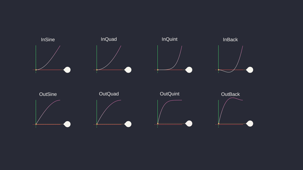
Let’s see some other function examples:

• In Sine: \(\sin(\frac{\pi}{2}t)\)
• In Quad: \(t^2\)
• In Cubic: \(t^3\)
• In Quart: \(t^4\)
• In Quint: \(t^5\)
• In Expo: \(2^{10(t-1)}\)
• In Circ: \(1 - \sqrt{1 - t^2}\)
• In Back: \(t^2(2.70158t - 1.70158)\)
• In Elastic: \(2^{10(t-1)} * \sin(13\pi t)\)
• In Bounce: \(1 - \cos(\frac{\pi}{2}t)\)

You can also test by yourself the different easing functions in the previous graph.

Flip

Flipping an easing function reverses its progression, creating an opposite direction effect. Mathematically, to flip a linear easing function \(y = x\), subtract the input value x from 1: \(y = 1 - x\).

float Flip(float t) => 1 - t;

Ease out

For a rocket landing, we want the rocket to start fast and end slow. To achieve this, we can use flip the quadratic function. With that, we just discovered the ease out function, that starts fast and ends slow.

After applying it to a quadratic function, we get: \(f(t) = (1 - t)^2\).

However, we need it to start at 0 and end at 1, so we need to flip it again, resulting in a proper ease out function: \(f(t) = 1 - (1 - t)^2\)

float OutQuad(float t) => Flip( InQuad( Flip( t ) ) );

Some ease out function examples:

• Out Sine: \(\sin(\frac{\pi}{2}t)\)
• Out Quad: \(1 - (1 - t)^2\)
• Out Cubic: \(1 - (1 - t)^3\)
• Out Quart: \(1 - (1 - t)^4\)
• Out Quint: \(1 - (1 - t)^5\)
• Out Expo: \(1 - 2^{-10t}\)
• Out Circ: \(\sqrt{1 - (t - 1)^2}\)
• Out Back: \(1 - (1 - t)^2(2.70158(1 - t) - 1.70158)\)
• Out Elastic: \(1 - 2^{-10t} \sin(13\pi(2t - 0.5))\)
• Out Bounce: \(\cos(\frac{\pi}{2}t)\)

Ease in out

If we want to combine both effects, we can use the ease in out function, that merges the ease in and ease out functions.

float InOutQuad(float t) => t < 0.5F
                            ? InQuad( t ) * 2
                            : Flip( InQuad( -2 * t + 2 ) ) / 2;

Alternatively, we can lerp between the ease in and ease out functions.

float InOutQuad(float t) => Lerp( InQuad( t ), OutQuad( t ), t );

Enhancing the lerp technique

But what if we want a function that can express a lot of different movements in a easy way? We can use a cubic polynomial¹!

To achieve this, we need to ensure that the function always starts at 0 and ends at 1.

Here are the steps to define the function:

• Start with the initial function: \(f(t) = at^3 + bt^2 + ct + d\)
• We want the graph to start at 0, so we set \(f(0) = 0\):

\[\eqalign{ f(0) & = a(0)^3 + b(0)^2 + c(0) + d \\ f(0) & = 0 + 0 + 0 + d \\ d & = 0 }\]

• The updated function becomes: \(f(t) = at^3 + bt^2 + ct\)

• We want the graph to end at 1, so we set \(f(1) = 1\):

\[\begin{aligned} f(1) & = a(1)^3 + b(1)^2 + c(1) \\ f(1) & = a + b + c \\ 1 & = a + b + c \end{aligned}\]

• Since \(f(1)\) should equal 1, we have: \(c = 1 - a - b\)

• We can rewrite \(c\) as \((1 - a - b)\) and substitute it back into the function:

\[f(t) = at^3 + bt^2 + (1 - a - b)t\]

Now, the function \(f(t) = at^3 + bt^2 + (1 - a - b)t\) satisfies the conditions of starting at (0,0) and ending at (1,1) for any given values of \(a\) and \(b\).

That’s it! We can now pass any values of \(a\) and \(b\) to the function to create different easing effects:

• Linear: we can set \(a\) and \(b\) to 0.
• In Back: we can set \(a\) as 1.5 and \(b\) as 0.
• Out Back: we can set \(a\) as 1.25 and \(b\) as -4.

float Custom(float t, float a, float b)
{
  float c = 1 - a - b;
  return ( a * t * t * t ) + ( b * t * t ) + ( c * t );
}

Try to play with the values in this Desmos graph.

Embrace the Easing Frontier

Is that all? Not even close! The world of easing functions is vast and full of possibilities. There’s so much more to explore and experiment with.

You have the ability to create your own mathematical functions, giving birth to unique and captivating easing effects. Combine different functions together, and witness the magic that unfolds as your animations come to life.

But wait, there’s more! Have you heard about Splines and Bezier Curves? These intriguing techniques call for your curiosity to dive deeper into uncharted territory.

May you live long and animate with great success!

1. Cubic equation. Available in: https://en.wikipedia.org/wiki/Cubic_equation. ↩